.png?alt=media&token=78eaee3a-6189-4df0-8557-c268ef81bf1b)
Scene overview
Scene overview
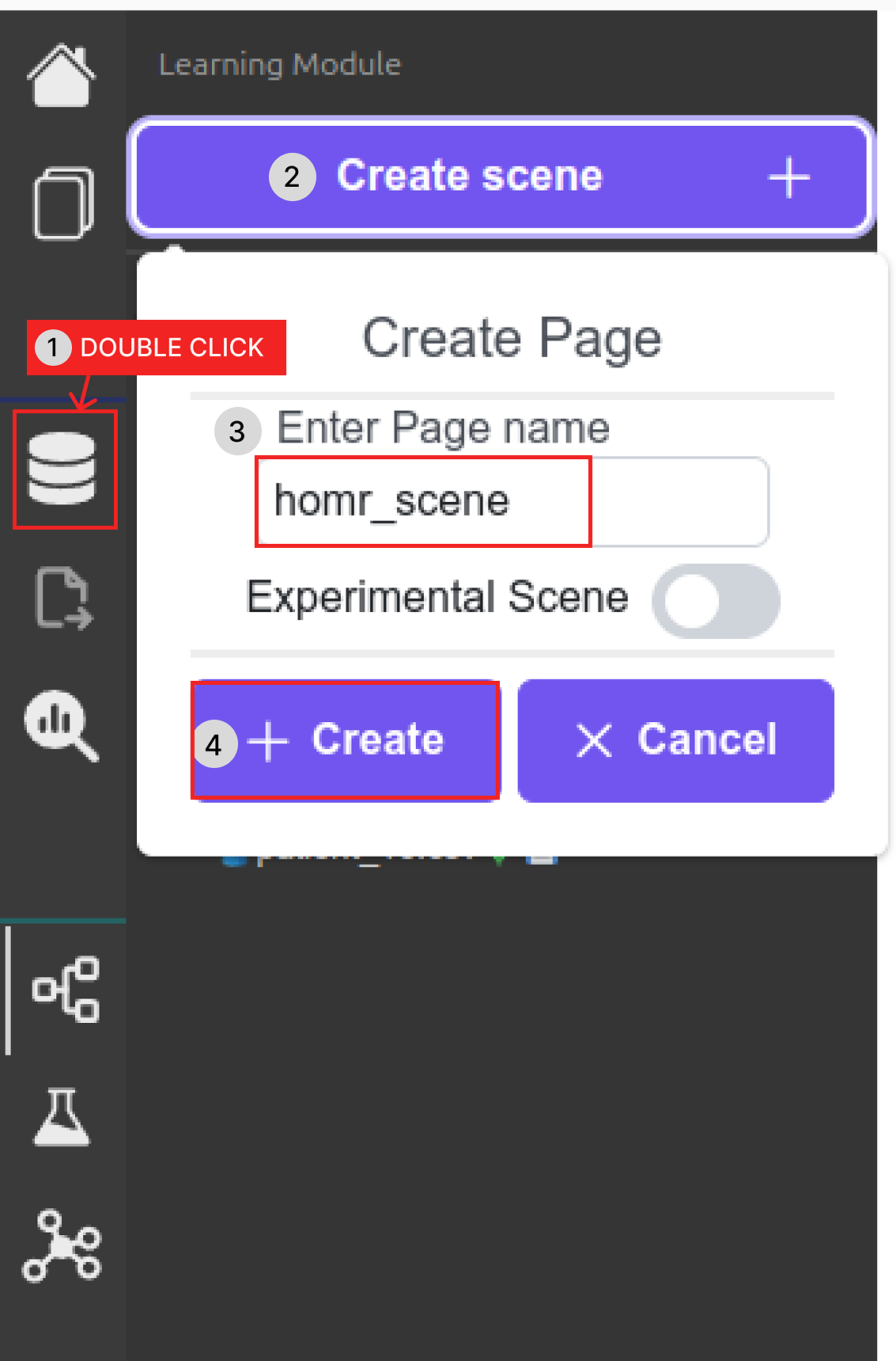
Create the "homr_scene" scene
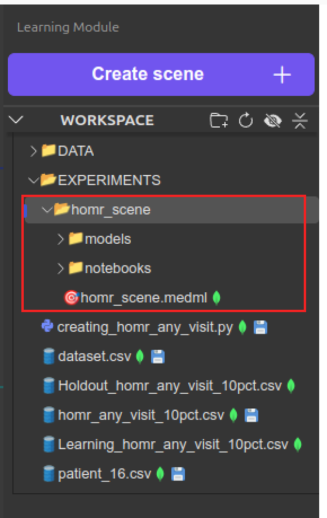
homr_scene folder in Experiments
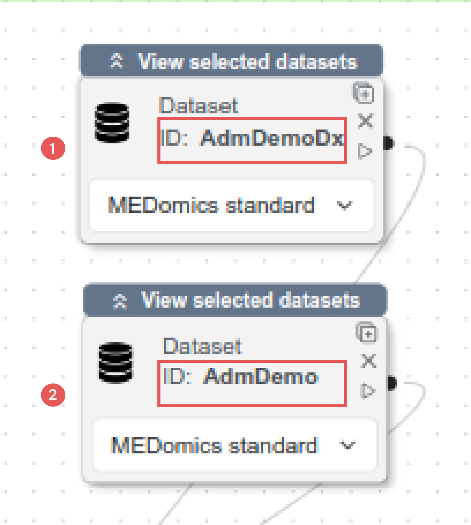
Dataset Nodes setup
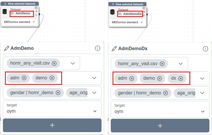
Dataset Nodes configuration
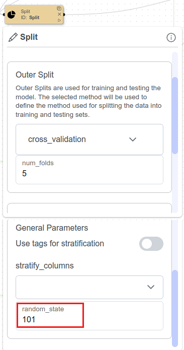
Split Node configuration
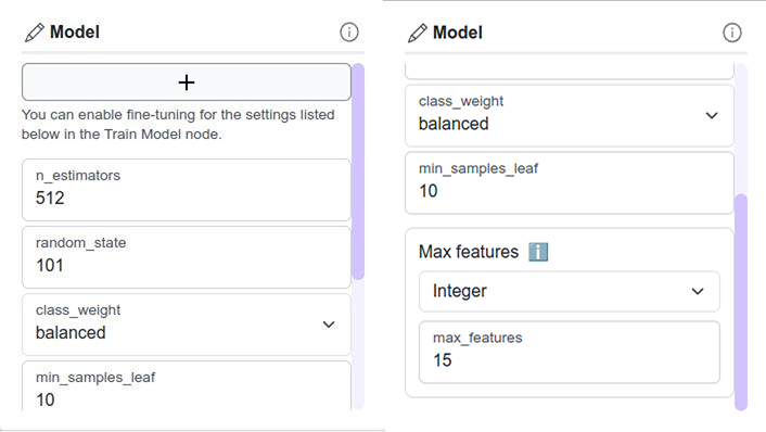
Model Hyperparameters configuration
.png?alt=media&token=747a79a1-11d3-42ae-abb2-a3ceec36e422)
Train Model Node setup
.png?alt=media&token=5219648e-bc0b-4a93-9c67-a4715f79cf27)
Custom Tuning Grid for our model
.png?alt=media&token=8f4037de-78bb-4305-a590-affab986c613)
Tune Model options
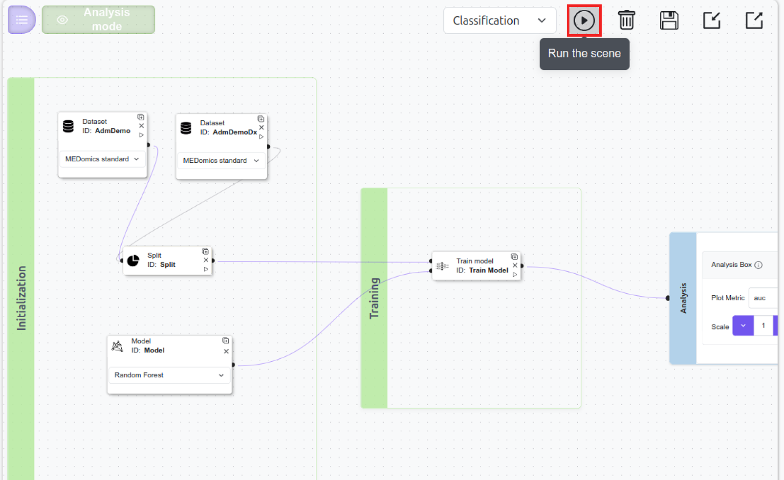
Run the scene
.png?alt=media&token=15ad0dc8-9f33-4db8-b256-52416d3971dd)
Pipeline results in Analysis Mode
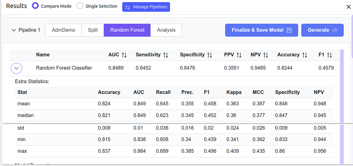
Metrics' statistics for the AdmDemo model
.png?alt=media&token=2af41fa5-6e5e-4edc-8a7f-9b3bd61ca146)
Metrics' statistics for the AdmDemoDx model
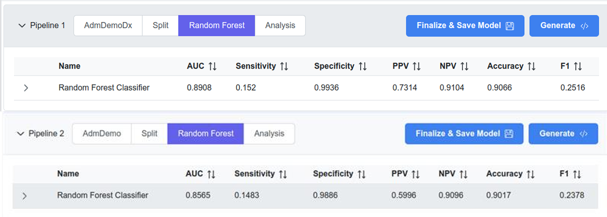
AdmDemo and AdmDemoDx results